Measuring the particle size distribution (PSD) of ground calcium carbonate is a critical step in evaluating grinding efficiency, product quality, and suitability for specific applications. Currently, several standardized and high-precision methods are used in both industrial and laboratory settings, with laser diffraction being the most widely adopted. The details are as follows:
1. Primary Method: Laser Diffraction (Laser Particle Size Analysis)
✅ Principle
Based on Fraunhofer diffraction or Mie scattering theory: particles of different sizes scatter laser light at different angles. By detecting the angular intensity distribution of scattered light, the instrument calculates the particle size distribution.
✅ Advantages
Wide measurement range: 0.01 μm – 3.500 μm (covers nano- to millimeter-scale particles)
Fast analysis: single measurement takes only 10–60 seconds
High repeatability: relative standard deviation (RSD) < 1%
Supports both dry and wet dispersion (using water, ethanol, etc.)
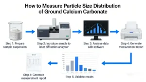
✅ Typical Procedure (Wet Dispersion Method):
Sample Preparation: Weigh a small amount (~0.1 g) of ground calcium carbonate powder.
Select Dispersant: Use deionized water with a small amount of dispersant (e.g., sodium hexametaphosphate or sodium citrate) to prevent agglomeration.
Ultrasonic Dispersion: Sonicate for 2–5 minutes in an ultrasonic bath to break up soft agglomerates.
Add to Measurement Cell: Adjust obscuration to 10%–20% to avoid multiple scattering.
Run Measurement: Use instruments such as Malvern Mastersizer, Horiba LA-960. or Bettersize BT-9300.
Output Results: Obtain key parameters like D₁₀, D₅₀ (median diameter), D₉₀, D₉₇, and the full distribution curve.
📌 Key Metrics:
D₅₀: 50% of particles are smaller than this value (represents average size)
D₉₇: 97% of particles are smaller than this value—commonly used in industrial specifications (e.g., “D₉₇ ≤ 10 μm”)
2. Alternative or Complementary Methods
| Method | Principle | Best For | Limitations |
|---|---|---|---|
| **Dynamic Light Scattering **(DLS) | Measures Brownian motion of nanoparticles | Nano-CaCO₃ (<1 μm) | Insensitive to micrometer-sized particles; skewed by large aggregates |
| **Scanning Electron Microscopy **(SEM) | High-resolution imaging via electron beam | Visualizing particle morphology and agglomeration | Does not provide statistical distribution directly; requires image analysis software (e.g., ImageJ) |
| **Sedimentation **(Gravity/Centrifugal) | Based on Stokes’ law: settling velocity ∝ particle size | Coarse powders (>45 μm); low-cost labs | Time-consuming (hours); low resolution; largely outdated |
| Sieve Analysis | Mechanical sieving through standard mesh | Very coarse grades (>45 μm, e.g., below 325 mesh) | Poor accuracy for fine powders; labor-intensive |
💡 Recommendation:
Routine QC → Laser diffraction (preferred)
Nano-grade R&D → DLS + TEM/SEM
Morphology validation → SEM to check for crystal damage from over-grinding

3. Critical Considerations for Accurate Results
Adequate Dispersion
CaCO₃ tends to agglomerate. Ultrasonication + dispersant is essential; otherwise, you measure agglomerates—not primary particles.
Correct Optical Parameters
Input accurate optical properties into the software:
Refractive Index: 1.58–1.66 (typically set to 1.59)
Absorption: 0.1–0.5 (use 0.1 for CaCO₃)
Eliminate Air Bubbles
In wet measurements, degas or stir gently to remove bubbles that scatter light falsely.
Regular Calibration
Calibrate the instrument periodically using certified reference materials (e.g., NIST-traceable latex microspheres).
4. Example Report (Ground Ground Calcium Carbonate)
| Parameter | Value |
|---|---|
| D₁₀ | 1.8 μm |
| D₅₀ | 4.2 μm |
| D₉₀ | 8.5 μm |
| D₉₇ | 10.3 μm |
| BET Surface Area | 3.2 m²/g |
| Distribution Span | (D₉₀ − D₁₀)/D₅₀ ≈ 1.58 (moderately narrow) |
✅ Span < 1.0: very narrow distribution
✅ Span > 1.5: broad distribution
Conclusion
Laser diffraction is the gold standard for measuring the particle size distribution of ground calcium carbonate, offering speed, wide dynamic range, and excellent reproducibility.
The key to reliable data lies in proper sample dispersion and correct instrument settings. Combining laser analysis with SEM imaging provides a comprehensive view of both size and morphology, enabling optimization of grinding parameters (e.g., mill speed, duration, grinding aids).