Fineness control is critical in mineral processing (e.g., calcium carbonate, graphite for lithium battery applications) and other industries. This guide provides detailed procedures for two primary methods—sieve analysis (traditional, cost-effective, ideal for coarse-to-medium particles) and laser diffraction (advanced, high-resolution, optimal for fine particles and full distributions) .
1. Sieve Analysis: Step-by-Step Procedure
Equipment Requirements
- Set of standard test sieves (ISO 3310, ASTM E11) with decreasing aperture sizes ASTM
- Sieve shaker (mechanical or electromagnetic)
- Calibrated analytical balance (precision: ±0.1 mg)
- Collection pan (receiver)
- Brush for cleaning sieves
- Sample splitter (riffler) for representative sampling
- Drying oven (if sample is moist)
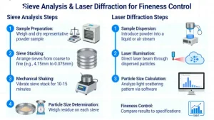
Step 1: Sample Preparation
- Dry the sample at 105°C (if moisture content >5%) to prevent agglomeration and sieve blockage
- Use a sample splitter to obtain a representative sub-sample (50–500 g, depending on particle size: larger particles need larger samples)
- Weigh the prepared sample (W₀) and record the value (precision: ±0.01 g)
Step 2: Sieve Stack Assembly
- Inspect and clean all sieves for damage (bent wires, blocked apertures)
- Arrange sieves in descending order of aperture size: largest on top, smallest above the collection pan
- Weigh and record the empty weight of each sieve and the collection pan (W_sieve, W_pan)
Step 3: Sieving Process
- Place the prepared sample on the top sieve
- Cover the stack with a lid and secure in the sieve shaker
- Set shaking parameters:
- Time: 10–15 minutes (mechanical), 5 minutes (high-efficiency shakers)
- Amplitude: 1–3 mm (adjust based on material type)
- Optional: Tap frequency for difficult-to-sieve materials
- Start the shaker and monitor progress
Step 4: Post-Sieving Analysis
- Disassemble the stack carefully, starting from the top
- Weigh each sieve with retained material (W_total) and calculate the net weight retained: W_retained = W_total – W_sieve
- Weigh the collection pan with fines: W_fines = W_pan_total – W_pan
- Mass balance check: Sum of all fractions should be within ±1–2% of initial sample weight (W₀)
Step 5: Data Calculation
| Parameter | Formula | Purpose |
|---|---|---|
| % Retained | (W_retained / W₀) × 100 | Percentage of particles larger than sieve aperture |
| Cumulative % Retained | Sum of % retained on current and all coarser sieves | Progressive oversize material |
| Cumulative % Passing | 100 – Cumulative % Retained | Fineness index (e.g., D₅₀ = particle size where 50% passes) |
Step 6: Reporting
- Tabulate results with sieve sizes, individual weights, and calculated percentages
- Plot particle size distribution curve: log(particle size) vs. cumulative % passing
- Report key fineness metrics: D₁₀, D₅₀, D₉₀ (10%, 50%, 90% passing sizes) and span (D₉₀-D₁₀/D₅₀)
2. Laser Diffraction: Step-by-Step Procedure
Equipment Requirements
- Laser diffraction particle size analyzer (e.g., Malvern Mastersizer, Sympatec HELOS)
- Dispersion unit (dry or wet):
- Dry: for free-flowing powders, uses compressed air
- Wet: for cohesive materials, uses liquid medium (water, ethanol, etc.)
- Sample preparation tools (spatula, beakers, ultrasonic probe for deagglomeration)
- Refractive index data for sample and dispersion medium
Principle of Operation
Laser diffraction measures angular variation in scattered light intensity as a laser beam passes through a dispersed sample :
- Large particles: scatter light at small angles
- Small particles: scatter light at large angles
- The instrument uses Mie theory (or Fraunhofer approximation for large particles) to calculate particle size distribution based on volume-equivalent spheres
Step 1: Instrument Setup
- Power on the analyzer and allow 30 minutes for warm-up and stabilization
- Select appropriate optical model:
- Mie theory: for particles <100 µm, requires refractive index (RI) of sample and medium
- Fraunhofer: for particles >100 µm, no RI needed but less accurate for irregular shapes
- Configure dispersion parameters:
- Dry: air pressure, feed rate, measurement time
- Wet: stirring speed, sonication time (if needed), pump flow rate
- Perform background measurement to account for dispersion medium alone
Step 2: Sample Preparation
- Dry samples: Ensure moisture content <1% to prevent agglomeration
- Wet samples:
- Select a compatible dispersion medium (no chemical reaction with sample)
- Add dispersant if needed (e.g., 0.1% sodium hexametaphosphate for minerals) to prevent re-agglomeration
- Prepare a dilute suspension (typically 0.1–1% solids) to avoid multiple scattering
Step 3: Measurement Process
- Inject sample into the measurement zone:
- Dry: Use a powder feeder to introduce sample into the air stream
- Wet: Pipette or pour the suspension into the circulation system
- Monitor the obscuration level (5–20% is optimal) to ensure proper concentration
- Perform 3–5 replicate measurements for statistical reliability
- Clean the system thoroughly between samples to prevent cross-contamination
Step 4: Data Analysis
- The instrument automatically calculates:
- Particle size distribution (PSD) in volume %
- Key metrics: D₁₀, D₅₀, D₉₀, span, and specific surface area
- Validate results:
- Check reproducibility: coefficient of variation (CV) for D₅₀ should be <3% ISO
- Compare with sieve analysis for overlapping size ranges (40–1000 µm)
Step 5: Reporting
- Generate a comprehensive report including:
- Instrument model and settings (optical model, dispersion parameters)
- Refractive index values used
- Raw data (PSD table)
- Graphical representation (PSD curve, cumulative distribution)
- Key fineness parameters with statistical confidence intervals ISO
3. Sieve Analysis vs. Laser Diffraction: Key Differences for Fineness Control
| Aspect | Sieve Analysis | Laser Diffraction | Best For |
|---|---|---|---|
| Size Range | 40 µm – 100 mm (standard); lower limit ~20 µm with wet sieving | 0.01 µm – 3 mm (standard); extended ranges available ISO | Sieve: Coarse to medium particles
Laser: Fine particles, full distribution |
| Measurement Principle | Particle passage through mesh openings (minimum dimension) | Light scattering (volume-equivalent sphere diameter) | Sieve: Shape-sensitive applications
Laser: Volume-based fineness control |
| Analysis Time | 15–30 minutes per sample (including setup and cleaning) | 2–5 minutes per sample (automated) | Sieve: Low-throughput quality control
Laser: High-throughput process monitoring |
| Sample Amount | 50–500 g (larger for coarse particles) | 1–50 mg (dry), 1–10 mL suspension (wet) | Sieve: Bulk material verification
Laser: Limited sample availability |
| Accuracy/Repeatability | Moderate; affected by particle shape, sieve loading | High; less shape-dependent, automated | Sieve: Routine quality checks
Laser: Critical process control, research |
| Cost | Low (equipment and maintenance) | High (initial investment, maintenance) | Sieve: Budget-constrained operations
Laser: Advanced process optimization |
| Automation | Limited; manual weighing required | High; fully automated with software control | Sieve: Simple quality control
Laser: 24/7 process monitoring |
4. Practical Tips for Fineness Control in Grinding Operations
Sieve Analysis Best Practices
- Sieve selection: Choose a logarithmic sequence (e.g., 250, 125, 63, 32, 16 µm) for better PSD resolution
- Sieving time: Verify with the residue method: sieve for additional 2 minutes—if <0.5% additional material passes, sieving is complete
- Wet sieving: For particles <45 µm, use wet sieving with a dispersant to prevent agglomeration
- Cleaning: Brush sieves gently after each use; ultrasonic cleaning for blocked apertures
Laser Diffraction Best Practices
- Dispersion optimization:
- Dry: Adjust air pressure to deagglomerate without particle breakage
- Wet: Use ultrasonic treatment (1–3 minutes) for cohesive minerals like calcium carbonate
- Refractive index: Use accurate RI values (e.g., CaCO₃: 1.65, graphite: 2.7) for reliable Mie theory calculations
- Sample concentration: Maintain obscuration between 5–15% to avoid multiple scattering errors
- Method validation: Cross-check with sieve analysis for particles >40 µm to ensure consistency
Integration for Comprehensive Fineness Control
- Combine methods: Use sieve analysis for coarse fraction control and laser diffraction for fine particle characterization
- Process feedback: Establish control charts for D₅₀ and span to monitor grinding efficiency
- Calibration: Periodically calibrate both instruments with standard reference materials (e.g., NIST traceable glass beads) ISO
- SOP development: Create detailed standard operating procedures for consistent results across operators
5. Troubleshooting Common Issues
| Problem | Sieve Analysis | Laser Diffraction |
|---|---|---|
| Poor reproducibility | Uneven sample loading; damaged sieves; insufficient sieving time | Inadequate dispersion; inconsistent obscuration; dirty optics |
| Mass loss >2% | Material adhesion to sieves; sample spillage; static electricity | Sample adsorption to cell walls; incomplete recovery |
| Unexpectedly coarse results | Sieves blocked by agglomerates; incorrect sieve order | Insufficient sonication; incorrect refractive index |
| Unexpectedly fine results | Sieves damaged (enlarged apertures); over-sieving (particle breakage) | Excessive sonication (particle breakage); multiple scattering |
Summary
- Sieve analysis is ideal for routine quality control of coarse-to-medium particles (40 µm–100 mm), offering simplicity and cost-effectiveness
- Laser diffraction excels in fine particle characterization (0.01 µm–3 mm), providing high-resolution PSD data essential for advanced process optimization ISO
- For comprehensive fineness control in grinding operations, combine both methods: use sieve analysis for process monitoring of coarse fractions and laser diffraction for detailed fine particle characterization and research applications .